基于LLRFLibsPy库的RF腔控制回路设置、建模和反馈控制设计

source code: Github

这段Python代码主要用于模拟一个RF腔控制回路的参数设置、建模和反馈控制设计。代码依赖于多个自定义模块(如set_path, rf_sim, rf_control, rf_calib, rf_sysid, rf_noise),这些模块应已被作者预先定义。下面是对代码的详细解释:

1. 导入库和模块

1
2
3
4
5
6
7
8
9
import numpy as np
import matplotlib.pyplot as plt

from set_path import *
from rf_sim import *
from rf_control import *
from rf_calib import *
from rf_sysid import *
from rf_noise import *

导入了基础的科学计算库numpy和绘图库matplotlib.pyplot,以及自定义文件中的必要模块。

2. 定义仿真参数

1
2
3
4
5
6
7
8
9
10
11
12
13
14
15
16
17
18
19
20
21
22
f_scale = 6                # 采样频率缩放因子,默认1MHz
pi = np.pi # π常量的简写
simN = 2048 * f_scale # 模拟RF脉冲时波形的点数

fs = 1e6 * f_scale # 采样频率,Hz
Ts = 1/fs # 采样时间,s

f0 = 1.3e9 # RF工作频率,Hz
roQ = 1036 # 腔体的r/Q值,Ohm
QL = 3e6 # 腔体的加载品质因数
RL = 0.5 * roQ * QL # 腔体加载阻抗(Linac约定),Ohm
ig = 0.016 # RF驱动功率等效电流,A
ib = 0.008 # 平均束流电流,A
t_fill = 510 * f_scale # 腔体填充周期的长度,样本数
t_flat = 800 * f_scale # 腔体平顶周期的长度,样本数

wh = pi*f0 / QL # 腔体的半带宽,rad/s
dw = wh # 腔体的失谐,rad/s

pb_modes = {'freq_offs': [-800e3], # 腔体传递带模式的偏移频率,Hz
'gain_rel': [-1], # 传递带模式相对π模式的增益
'half_bw': [2*np.pi*216 * 0.5]} # 传递带模式的半带宽,rad/s

这部分定义了采样频率、腔体参数、仿真周期等。
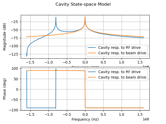
3. 定义腔体模型

1
2
3
4
5
result = cav_ss(wh, detuning = dw, passband_modes = pb_modes, plot = True)
Arf = result[1] # 腔体模型的状态空间矩阵
Brf = result[2]
Crf = result[3]
Drf = result[4]

使用cav_ss函数设置腔体模型,并获得其状态空间表示(A,B,C,D矩阵)。设置plot=True会显示频率响应图。
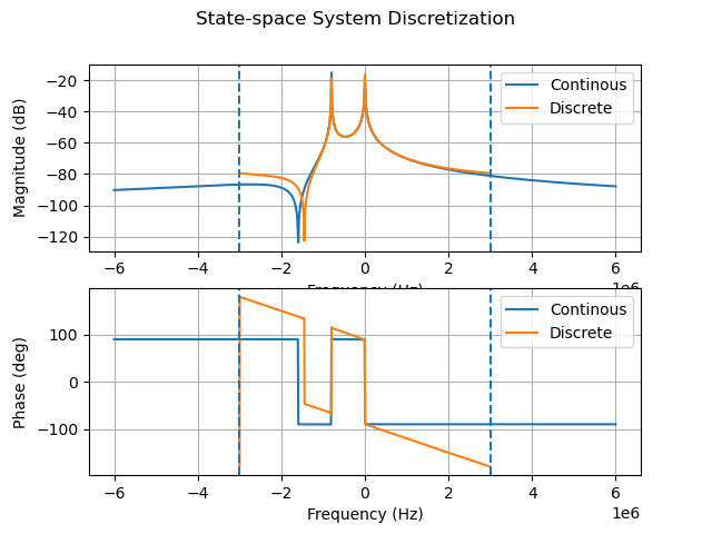
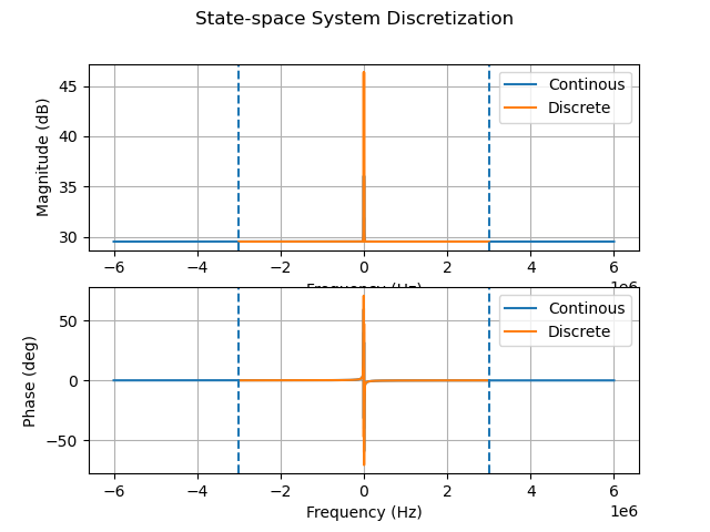
example-feedback-analysis-1.png

4. 离散化腔体方程

1
status1, Arfd, Brfd, Crfd, Drfd, _ = ss_discrete(Arf, Brf, Crf, Drf, Ts, method = 'zoh', plot = True)

使用ss_discrete函数将连续时间腔体方程离散化,并显示离散化后的频率响应。
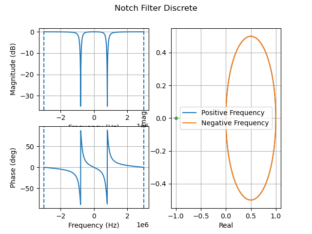
example-feedback-analysis-2.png

5. 设计一个陷波滤波器

1
2
status, Afd, Bfd, Cfd, Dfd = design_notch_filter(800e3, 4, fs)
ss_freqresp(Afd, Bfd, Cfd, Dfd, Ts = Ts, title = 'Notch Filter Discrete', plot = True)

设计一个陷波滤波器以移除测量中的传递带模式,并显示其频率响应。
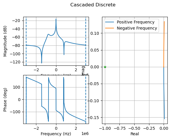
example-feedback-analysis-3.png

6. 级联腔体模型和陷波滤波器

1
2
status, AGd, BGd, CGd, DGd, _ = ss_cascade(Arfd, Brfd, Crfd, Drfd, Afd, Bfd, Cfd, Dfd, Ts = Ts)
ss_freqresp(AGd, BGd, CGd, DGd, Ts = Ts, title = 'Cascaded Discrete', plot = True)

将腔体模型与陷波滤波器级联,形成要控制的对象,并显示其频率响应。
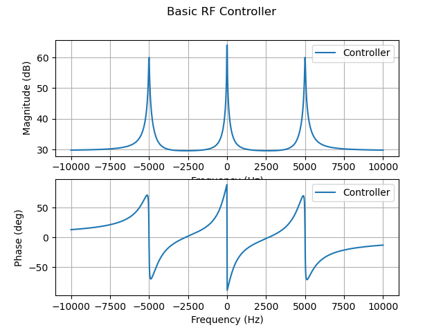
example-feedback-analysis-4.png

7. 定义反馈控制器

1
2
3
4
5
6
7
8
Kp = 30                                  # 比例增益
Ki = 1e5 # 积分增益

notches = {'freq_offs': [5e3], # 反馈控制器的陷波滤波器配置
'gain': [1000],
'half_bw': [2*np.pi*20]}

status, Akc, Bkc, Ckc, Dkc = basic_rf_controller(Kp, Ki, notch_conf = notches, plot = True, plot_maxf = 10e3)

定义一个基本的RF控制器,包括比例增益和积分增益,以及用于反馈环的陷波滤波器,设置plot=True显示频率响应图。

example-feedback-analysis-5.png

8. 离散化控制器

1
status, Akd, Bkd, Ckd, Dkd, _ = ss_discrete(Akc, Bkc, Ckc, Dkc, Ts, method = 'bilinear', plot = True, plot_pno = 10000)

将控制器离散化,并显示离散化后的频率响应。
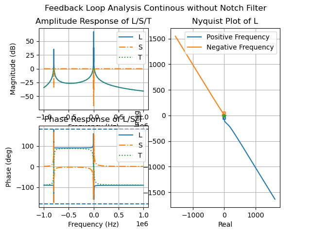
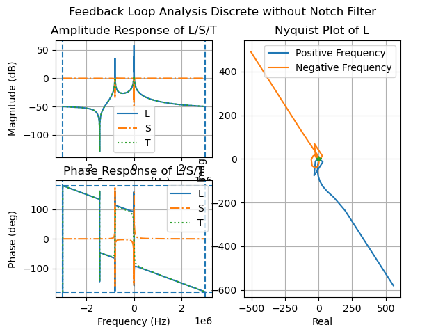
example-feedback-analysis-6.png

9. 计算回路特性

1
2
3
4
5
delay_s = 0  # 延迟将影响稳定性和裕度

rc = loop_analysis(Arf, Brf, Crf, Drf, Akc, Bkc, Ckc, Dkc, delay_s = delay_s, label = 'Continous without Notch Filter')
rd = loop_analysis(AGd, BGd, CGd, DGd, Akd, Bkd, Ckd, Dkd, Ts = Ts, delay_s = delay_s, label = 'Discrete with Notch Filter')
rd2 = loop_analysis(Arfd, Brfd, Crfd, Drfd, Akd, Bkd, Ckd, Dkd, Ts = Ts, delay_s = delay_s, label = 'Discrete without Notch Filter')

计算开环响应、灵敏度和互补灵敏度等回路特性,并标记分析结果。

example-feedback-analysis-7.png

image.png

example-feedback-analysis-9.png

总结来说,这段代码搭建了一个RF腔模拟控制系统,包括腔体模型、反馈控制器的设计与离散化,并进行了回路分析以评估系统性能。