基于LLRFLibsPy库的迭代学习控制算法优化脉冲超导腔前馈信号

source code: Github

这段代码用于模拟一个射频(RF)腔体控制回路。它包含定义参数、建立腔体模型、识别腔体的脉冲响应、使用迭代学习控制(ILC)设计控制器并进行模拟的过程。以下是代码的详细解读:

导入库和定义路径

1
2
3
4
5
6
7
8
import numpy as np
import matplotlib.pyplot as plt

from set_path import *
from rf_sim import *
from rf_calib import *
from rf_sysid import *
from rf_control import *
  • 导入必要的库和模块。numpy用于数值计算,matplotlib用于绘图,其余导入的是特定的射频模拟和控制模块。

定义腔体控制回路模拟参数

1
2
3
4
5
6
7
8
9
10
11
12
13
14
15
16
17
18
19
20
21
22
23
24
25
26
f_scale = 1                         # 采样频率缩放因子
pi = np.pi # 更短的 pi 表示
simN = 2048 * f_scale # 模拟射频脉冲的波形点数

# 腔体参数
fs = 1e6 * f_scale # 采样频率,Hz
Ts = 1/fs # 采样时间,s

f0 = 1.3e9 # 射频工作频率,Hz
roQ = 1036 # 腔体的r/Q值,Ohm
QL = 3e6 # 腔体的加载品质因数
RL = 0.5 * roQ * QL # 腔体的加载电阻,Ohm
ig = 0.016 # 射频驱动功率等效电流,A
ib = 0.008 # 平均束流电流,A
t_fill = 510 * f_scale # 腔体填充期的长度,采样点数
t_flat = 800 * f_scale # 腔体平顶期的长度,采样点数
t_bms = 600 * f_scale # 束流脉冲开始时间,采样点数
t_bme = 1000 * f_scale # 束流脉冲结束时间,采样点数

vc0 = 25e6 # 平顶腔体电压,V
wh = pi*f0 / QL # 腔体的半带宽,rad/s
dw = wh # 腔体的失谐频率,rad/s

pb_modes = {'freq_offs': [-800e3], # 腔体通带模式的偏移频率,Hz
'gain_rel': [-1], # 相对于 pi 模式的增益
'half_bw': [2*np.pi*216 * 0.5]} # 通带模式的半带宽,rad/s
  • 定义了射频腔体的基本参数,包括采样频率、工作频率、r/Q值、品质因数、加载电阻、驱动电流、束流电流以及腔体的各种时间常数和频率参数。

推导设定点和前馈

1
2
3
4
5
6
7
8
# 推导设定点和前馈
status, vc_sp, vf_ff, vb, T = cav_sp_ff(wh, t_fill, t_flat, Ts,
vc0 = vc0,
detuning = 0,
pno = simN)

vb = np.zeros(simN, dtype = complex) # 初始化束流驱动电压,V
vb[t_bms:t_bme] = -RL * ib # 设置束流驱动电压
  • 通过调用cav_sp_ff函数推导腔体的设定点和前馈信号,并初始化束流驱动电压。

定义腔体模型

1
2
3
4
5
6
7
8
9
10
11
12
13
14
15
16
17
18
19
20
# 定义腔体模型
result = cav_ss(wh, detuning = dw, passband_modes = None, plot = False)

status = result[0]
Arf = result[1] # 射频驱动的状态空间模型
Brf = result[2]
Crf = result[3]
Drf = result[4]
Abm = result[5] # 束流驱动的状态空间模型
Bbm = result[6]
Crf = result[7]
Dbm = result[8]

# 使用给定前馈信号模拟腔体的响应
status, T1, vc1, vr1 = sim_ncav_pulse(Arf, Brf, Crf, Drf, vf_ff, Ts,
Abmc = Abm,
Bbmc = Bbm,
Cbmc = Cbm,
Dbmc = Dbm,
vb = vb)
  • 定义腔体模型并通过调用cav_ss函数生成射频驱动和束流驱动的状态空间模型。
  • 使用前馈信号模拟腔体的响应。

离散化腔体方程

1
2
3
4
5
6
7
# 离散化腔体方程
status1, Arfd, Brfd, Crfd, Drfd, _ = ss_discrete(Arf, Brf, Crf, Drf, Ts,
method = 'zoh',
plot = False)
status2, Abmd, Bbmd, Cbmd, Dbmd, _ = ss_discrete(Abm, Bbm, Cbm, Dbm, Ts,
method = 'bilinear',
plot = False)
  • 使用ss_discrete函数离散化腔体的状态空间方程,便于数字控制。

识别腔体脉冲响应

1
2
3
4
5
6
7
8
9
10
11
12
13
14
15
16
# 识别腔体脉冲响应
status, h = cav_impulse(wh, dw, Ts, order = 2000)

# 使用最小二乘法识别脉冲响应
nwf = 200 # 波形数目
U = np.zeros((nwf, simN), dtype = complex) # 腔体输入波形
Y = np.zeros((nwf, simN), dtype = complex) # 腔体输出波形

for i in range(nwf):
# 随机输入
U[i] = np.random.normal(0.0, 1.0, simN) + 1j * np.random.normal(0.0, 1.0, simN)

# 模拟腔体输出
status, _, Y[i], _ = sim_ncav_pulse(Arf, Brf, Crf, Drf, U[i], Ts)

status, h2 = iden_impulse(U, Y, order = 2000)
  • 调用cav_impulse函数计算理论脉冲响应。
  • 使用最小二乘法从模拟数据中识别脉冲响应。

绘制脉冲响应结果

1
2
3
4
5
6
7
8
9
10
11
12
13
14
15
# 绘制脉冲响应结果
plt.figure()
plt.subplot(1,2,1)
plt.plot(np.abs(h))
plt.plot(np.abs(h2), '--')
plt.xlabel('No. of Sample')
plt.ylabel('Impul. Resp. Ampl.')
plt.grid()
plt.subplot(1,2,2)
plt.plot(np.angle(h, deg=True))
plt.plot(np.angle(h2, deg=True), '--')
plt.grid()
plt.xlabel('No. of Sample')
plt.ylabel('Impul. Resp. Phas. (deg)')
plt.show(block = False)
  • 绘制理论脉冲响应和识别的脉冲响应的幅值和相位对比图。

设计ILC矩阵

1
2
3
# 设计ILC矩阵
M = t_fill + t_flat # 矩阵的维度
status, L = AFF_ilc_design(h*2, M, P = np.eye(M)*50.0, Q = np.eye(M)*1.0)
  • 设计ILC矩阵L,用于后续的迭代学习控制。

模拟ILC

1
2
3
4
5
6
7
8
9
10
11
12
13
14
15
16
17
18
19
20
21
22
23
24
25
26
27
28
29
30
31
32
33
34
35
36
37
38
39
40
41
42
43
44
45
46
47
48
# 模拟ILC
vc2 = np.zeros(simN, dtype = complex) # 腔体输出,V
vaff = np.zeros(simN, dtype = complex) # 前馈信号,V

for pul_id in range(10): # 检查不同迭代的结果
print('Simulate pulse {}'.format(pul_id))

# 初始化腔体模拟器和控制器的状态
state_rf = np.matrix(np.zeros(Brfd.shape), dtype = complex)
state_bm = np.matrix(np.zeros(Bbmd.shape), dtype = complex)

# 模拟一个脉冲
for i in range(simN):
# 更新腔体输出
status, vc2[i], _, state_rf, state_bm = sim_ncav_step(Arfd, Brfd, Crfd, Drfd, vaff[i], state_rf,
Abmd = Abmd,
Bbmd = Bbmd,
Cbmd = Cbmd,
Dbmd = Dbmd,


vb_step = vb[i],
state_bm0 = state_bm)
# ILC
vff_cor = AFF_ilc(vc_sp[:M] - vc2[:M], L) # 使用ILC进行前馈校正
vaff[:M] = vaff[:M] + vff_cor
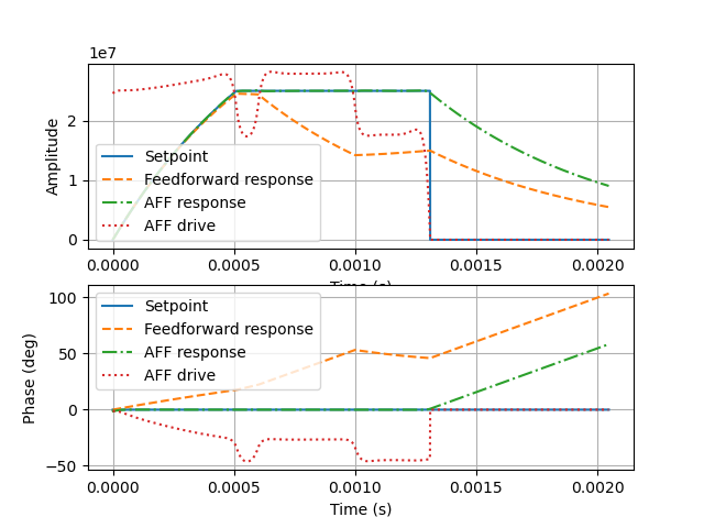
 # 更新前馈信号

# 绘制结果
plt.figure();
plt.subplot(2,1,1)
plt.plot(T, np.abs(vc_sp), label = 'Setpoint')
plt.plot(T, np.abs(vc1), '--', label = 'Feedforward response')
plt.plot(T, np.abs(vc2), '-.', label = 'AFF response')
plt.plot(T, np.abs(vaff), ':', label = 'AFF drive')
plt.legend()
plt.grid()
plt.xlabel('Time (s)')
plt.ylabel('Amplitude')
plt.subplot(2,1,2)
plt.plot(T, np.angle(vc_sp,deg = True), label = 'Setpoint')
plt.plot(T, np.angle(vc1, deg = True), '--', label = 'Feedforward response')
plt.plot(T, np.angle(vc2, deg = True), '-.', label = 'AFF response')
plt.plot(T, np.angle(vaff, deg = True), ':', label = 'AFF drive')
plt.legend()
plt.grid()
plt.xlabel('Time (s)')
plt.ylabel('Phase (deg)')
plt.show(block = False)
  • 模拟ILC过程,并绘制各个迭代过程中腔体输出、设定点、前馈响应和前馈驱动的幅值和相位变化情况。

example-aff-ilc-1.png

example-aff-ilc-2.png

总结

这段代码实现了射频腔体的建模、响应模拟、脉冲响应识别、ILC矩阵设计和ILC模拟的完整流程。通过ILC迭代,可以逐步优化前馈信号,使腔体输出更接近设定点。