LLRFLibsPy库中cav_par_pulse函数解读
source code: Github
这个函数cav_par_pulse的主要作用是计算在射频(RF)脉冲期间,带束流关闭(beam off)情况下的驻波腔体的半带宽和失谐频率。下面对函数的具体实现和参数进行详细解释。
函数签名和参数说明
1 | def cav_par_pulse(vc, vf, half_bw, Ts, beta=1e4): |
参数:
vc: numpy数组(复数),表示腔体探测信号波形(参考平面)。vf: numpy数组(复数),表示腔体前向信号波形(校准到与腔体探测信号相同的参考平面)。half_bw: 浮点数,腔体的半带宽(由衰减的早期部分得出),单位为rad/s。Ts: 浮点数,采样时间,单位为秒。beta: 浮点数,输入耦合因子(非超导腔体需要;对于超导腔体,可以使用默认值,或者如果需要更准确的校准,可以指定)。
返回值:
status: 布尔值,表示成功(True)或失败(False)。wh_pul: numpy数组,脉冲期间的半带宽,单位为rad/s。dw_pul: numpy数组,脉冲期间的失谐频率,单位为rad/s。
输入检查
1 | # check the input |
- 检查
vc和vf的形状是否相同。 - 检查
half_bw是否大于0。 - 检查
Ts是否大于0。 - 检查
beta是否大于0。
如果任何条件不满足,函数返回False和两个None。
使用腔体极坐标方程
1 | # use cavity polar equation |
- 根据输入耦合因子
beta计算得到vd。 - 计算
vc和vd的振幅和相位。
计算导数
1 | # derivative |
- 计算
vc振幅和相位随时间的导数,使用np.gradient方法计算导数,步长为采样时间Ts。
计算脉冲期间的半带宽和失谐频率
1 | # calculate the half-bandwidth and detuning |
- 根据腔体的极坐标方程和导数计算脉冲期间的半带宽
wh_pul和失谐频率dw_pul。
返回结果
1 | return True, wh_pul, dw_pul |
- 返回
True,以及计算得到的半带宽和失谐频率。
总结
这个函数通过直接求解腔体方程,计算在射频脉冲期间驻波腔体的半带宽和失谐频率。这对于理解和控制加速器中的射频系统非常重要。通过输入探测信号和前向信号的波形,以及其他必要的参数,可以得到脉冲期间的半带宽和失谐频率,从而有助于对腔体性能的分析和优化。
以下是一个示例,演示如何使用cav_par_pulse函数来计算在射频脉冲期间的驻波腔体的半带宽和失谐频率。
示例代码:
1 | import numpy as np |
示例解释:
- 导入必要的库:导入
numpy和matplotlib.pyplot用于计算和绘图。 - 定义
cav_par_pulse函数:直接使用之前解释的函数实现。 - 设置示例参数:
sampling_time: 采样时间,单位为秒。half_bandwidth: 半带宽,单位为rad/s。beta: 输入耦合因子。
- 生成示例波形:
time: 时间数组,从0到0.01秒,步长为采样时间。vc: 腔体探测信号,使用复指数函数生成,包含一个频率为50Hz的信号和一个衰减因子。vf: 腔体前向信号,使用复指数函数生成,包含一个频率为50Hz的信号。
- 调用函数计算:调用
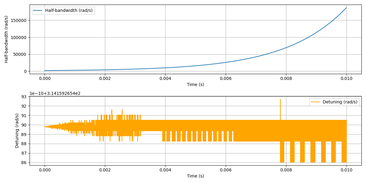
cav_par_pulse函数,传入示例波形和参数,计算半带宽和失谐频率。 - 打印和绘制结果:
- 如果计算成功,打印计算结果并绘制半带宽和失谐频率随时间变化的图像。
- 如果计算失败,打印失败信息。
运行此示例代码,将会看到脉冲期间的半带宽和失谐频率随时间的变化情况的图表。这有助于分析和理解腔体在射频脉冲期间的性能。